


In Matlab complex numbers can be created using x = 3 - 2i or x = complex(3, -2). The real part of a complex number is obtained by real(x) and the imaginary part by imag(x).
The complex plane has a real axis (in place of the x-axis) and an imaginary axis (in place of the y-axis). It is useful to plot complex numbers as points in the complex plane and also to plot function of complex variables using either contour or surface plots.
Plotting complex numbers
If the input to the Matlab plot command is a vector of complex numbers, the real parts are used as the x-coordinates and the imaginary parts as the y-coordinates.
The first argument is the real part, the second the imaginary part
Plotting the real and imaginary parts separately will work.
Matlab recognises the input is a complex number and does some of the work for you.
- specify a character ('*', '+', 'x', 'o', '.', etc) to be plotted at the point. help plot will give a list of available characters.
- use axis equal to ensure the real and imaginary axes have equal scales.
Define the vector z of the complex numbers. Note that -2+1i is equivalent to complex(-2,1), even if the variable i is defined to have a value other than sqrt(-1).
Plot the complex numbers in z as points.
You still need to add a grid and adjust the axes.

Eigenvalues of a real matrix
A real n by n matrix A has n eigenvalues (counting multiplicities) which are either real or occur in complex conjugate pairs.
Define a variable for the size of the matrix, and hence the number of eigenvalues.
Define an n by n matrix with elements taken from standard normal distribution.
Calculate the vector of n eigenvalues.
Plot the eigenvalues as points on the complex plane. Which eigenvalues are real and which are in a complex conjugate pair?
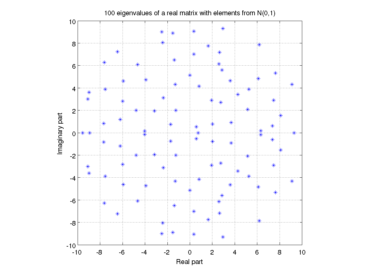
The MATLAB M-file used to create this plot is evplot.m.
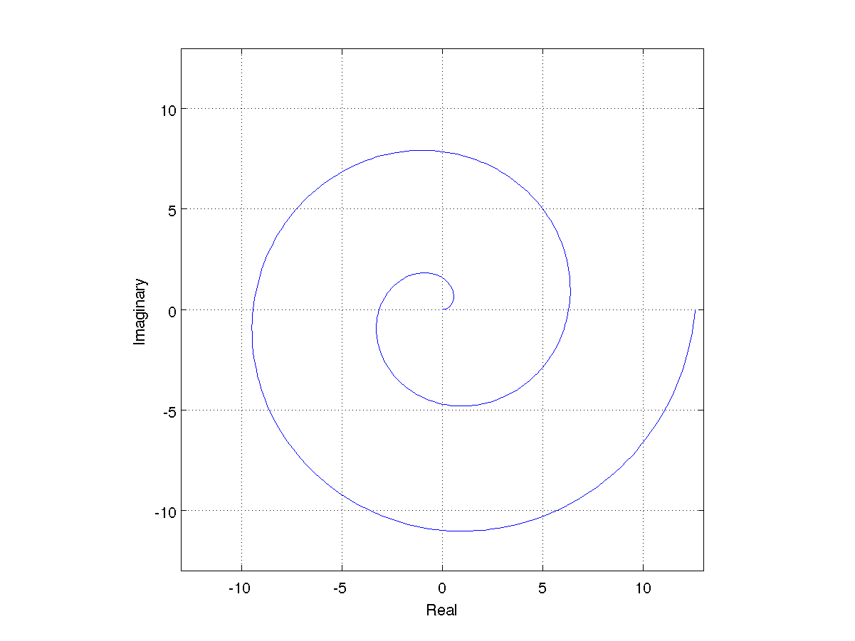
By default MATLAB joints each point (complex number) in the plot by a line segment, which for a fine grid of points gives a smooth curve.
Define a vector of 401 equally spaced points on the interval.
Calculate z using the MATLAB functions complex and exp.
Plot the elements of the vector z and join by line segments.
Ensure the real and imaginary axes have the same scaling.
Fix the axis limits.
Warnings
- What will happen if you use semilogx, semilogy or loglog to plot complex numbers? You may get Warning: Negative data ignored and only some subset of the points plotted.
- An expression of the form z = exp(i*t) may not work if the variable i has been redefined.
Self-test Exercise
Plot the complex curve z = e i t for t in [-4, 4]. What should the curve look like?Answer:
t = linspace(-4,4,401);
z = exp(complex(0,t));
plot(z);
The plot looks like an ellipse, but should be a circle with centre the origin and radius 1,
as |z| = 1 for all real t. To get a plot that looks like a circle, you need to make the axes equal.
Use the mouse to select the text between the word "Answer" and here to see the answer.
Summary
MATLAB can plot points or curves on an Argand diagram, using real and imaginary axes. You do not need to explicitly calculate the real and imaginary parts.