MATLAB Lesson 10 - More on plots

To visualise a function f(x, y) of two real variables we commonly use contour plots or surface plots (covered in the next topic).

Contours

A contour of a function f(x,y) of two variables is the set of points (x,y) where the function is constant. This is just the same as the height contours on a topographic map. Thus given a value a in the range of f, the corresponding contour is the set

C_a = { (x, y) : f(x, y) = a }.

If a is not in the range of the function f (for example a is less than the global minimum or greater than the global maximum of the function f) then the contour is the empty set.

Grids of points

Before a contour (or other 3-D plots) can be created, we need a rectangular array of function values F_i,j = f(x_j, y_i) at a grid of points x_j, j = 1,...,n and y_i, i = 1,...,m.

The easiest way to do this is to create arrays of grid points so that Matlab's elementwise operators can be used to evaluate the function.

To create arrays of grid points use the following three steps

Create a vector x of n grid points for the x variable;
Create a vector y of m grid points for the y variable;
Use the meshgrid function [X, Y] = meshgrid(x, y) to create arrays X, Y such that
X_i,j = x_j and Y_i,j = y_i for i = 1,...,m and j = 1,...,n.

The array X has the same value in each column, while the array Y has the same value in each row. Both X and Y will be m by n arrays (that is the number of elements in the first input argument to meshgrid determines the number of columns in the output arrays, while the number of elements in the second input vector argument determines the number of rows in the output arrays).

Create a vector x with 7 equally spaced points between -3 and 3, and a vector y with 9 equally spaced points between -4 and 4. Use the meshgrid function to create arrays X and Y.

Create the vector x of 7 equally spaced points on [-3, 3]

Create the vector y of 9 equally spaced points on [-4, 4]

Create the 9 by 7 arrays X and Y using the meshgrid function.

>> x = linspace(-3, 3, 7)

>> y = linspace(-4, 4, 9)

>> [X, Y] = meshgrid(x, y)

For this small example the commands have not been terminated with a semicolon, so the values are printed in the command window. For larger examples you definitely want to suppress output by adding a semicolon at the end of each line.

Note that the number number of elements in these vectors can be different, and the width of the intervals in the x and y directions does not have to be the same.

Arrays of function values

Having created arrays of grid points, we can use element wise operations to evaluate the function f at every element of X and Y producing an array F of the same size as X and Y.

Evaluate the function f(x, y) = x³ -3x + y² for each of the points in the arrays X, Y.

Use elementwise operator .^ to get the power of each element.

>> F = X.^3 - 3*X + Y.^2

A basic contour plot

Having created an array of function values, we can now used Matlab's contour function to visualise the function.

Use Matlab's contour function to plot contours of the data in the array F.

By default 10 contours are drawn.

>> contour(F)

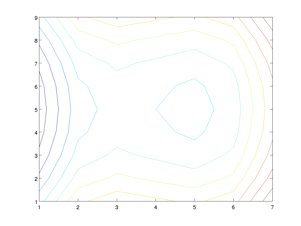
There are several things to note about this plot

The contours are not smooth. This could be a feature of the function, but more likely it is because not enough gird points have been used and Matlab is approximating a smooth curve by a sequence of straight lines.
The axes are labelled by the the row and column indices of the array F, not the values of x and y. It is not obvious that the function has a local minimum at (x,y) = (1,0) and a saddle point at (x,y)=(-1,0).
As always a title, axis labels and a grid should be added.
The value of each contour is not apparent.

A finer grid

To create a more realistic contour plot we need a finer grid of points and hence function values.

Create a vector x of 61 equally spaced points on [-3, 3] and a vector y of 81 equally spaced points on [-4, 4]. Use meshgrid to create arrays of grid points and evaluate the function f(x,y) = x^3 -3x + y^2 at each grid point.

Remember to use semicolons to suppress output.

Vector x of 61 equally spaced points on [-3,3].

Vector y of 81 equally spaced points on [-4,4].

Arrays (81 by 61) X and Y of grid points.

Array (81 by 61) F of function values.

>> x = linspace(-3, 3, 61);

>> y = linspace(-4, 4, 81);

>> [X, Y] = meshgrid(x, y);

>> F = X.^3 - 3*X + Y.^2;

A better contour plot

Create a contour plot with 25 contours of F using the vectors x and y for the axis labels, and add a grid and title.

Contour plot with 25 contours and axes determined by vectors x and y.

Add a grid to plot.

Add axis label for x-axis

Add axis label for y-axis

Add a title

>> contour(x, y, F, 25);

>> grid on;

>> xlabel('x');

>> ylabel('y');

>> title('f(x,y) = x^3 - 3 x + y^2');

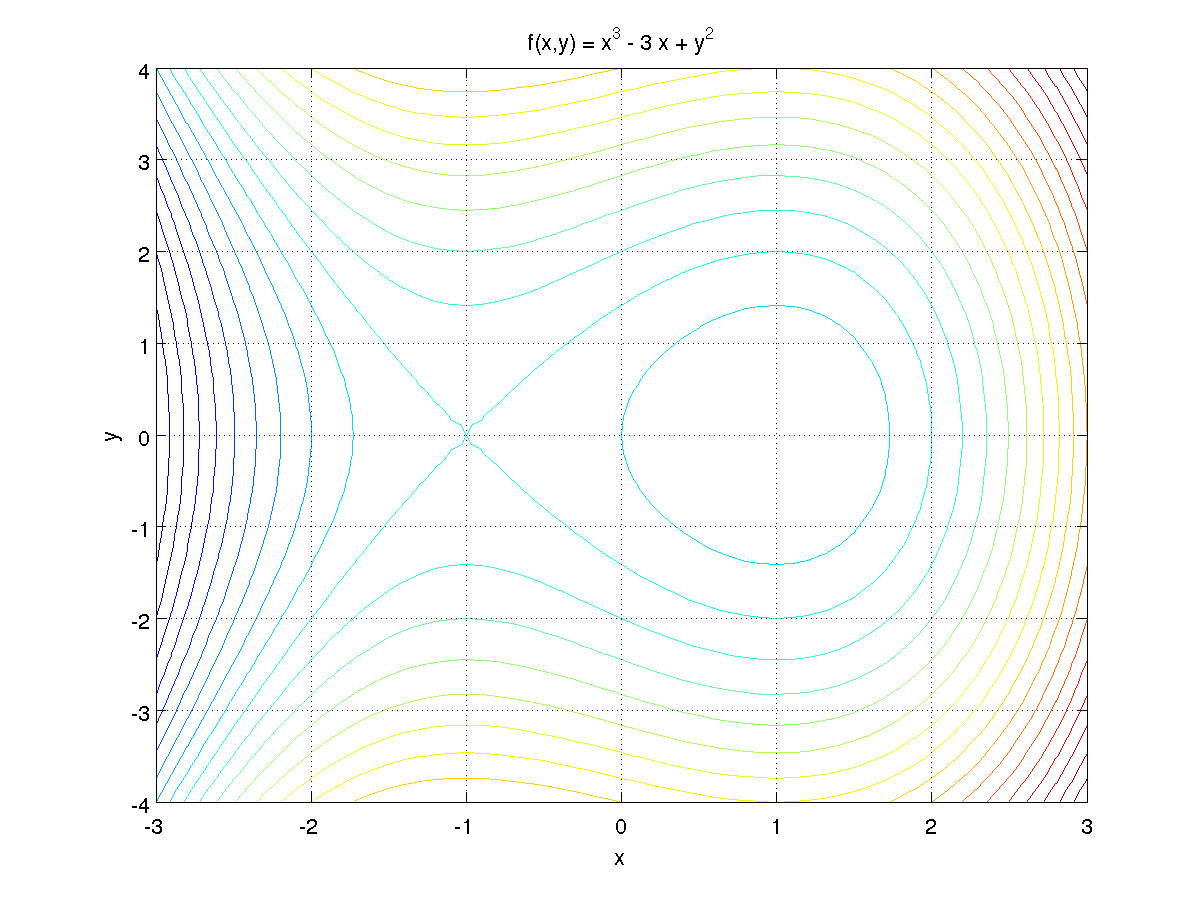
Now the contours are smooth, except possibly close to the point x = -1, y = 0, which is a saddle point of this function. An even finer grid will help make this clearer.

Contour labels

To add contour labels use the Matlab function clabel.

Create a contour plot of F with 15 contours and contour labels.

Contour plot using 15 contours with output for use in clabel.

Add labels to contours.

>> [c, h] = contour(x, y, F, 15);

>> clabel(c, h);

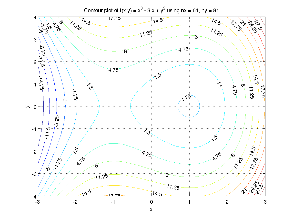
The command clabel(c, h, 'manual') allows you to put labels on contours clicked on with a mouse. Use Matlab's help facilities help contour or doc contour to get more information on these functions. For example, you can specify a vector of values for the contours instead of the number of contours.

The MATLAB M-file used to create these plots is plt3d.m.

Warnings

It is easy to get the values of x and y and which corresponds to the rows or columns of the array of function values incorrect. It is safer to use a different number of points in the x and y directions, as then Matlab will give an error message if the order is incorrect.

Self-test Exercise

Create a vector with elements

-10, -5, 0, 2, 4, 6, 8, 10, 15, 20, 25, 30

and plot the contours of the function f(x,y) = x^3 - 3 x + y^2 (the same as above) with these values.

Answer: Assuming x, y, F are as above:

cv = [-10 -5 0:2:10 15:5:30]
contour(x, y, F, cv)
Use the mouse to select the text between the word "Answer" and here to see the answer.

Summary

For functions of two variables, the meshgrid function will create arrays of grid points which can be used to evaluate a function using Matlab's elementwise operators. Then the contour function can be used to draw a contour plot of the function.

MATLAB Lesson 10 - Contour plots

Resources