


Plot command
In MATLAB you create a two dimensional plot using the plot command. The most basic form is
plot(x, y)
where x and y are vectors of the same length containing the data to be plotted.
Create a vector x of 401 equally spaced points on [0, 1]. Don't forget the final semicolon to suppress output!
Create a vector y of function values.
Plot the points, producing the figure below.
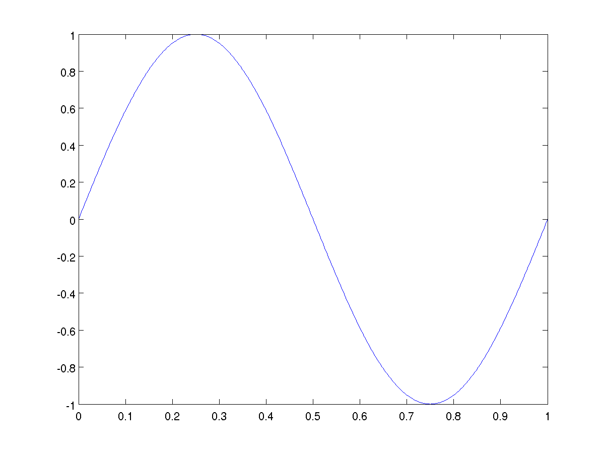
MATLAB's ability to evaluate functions of vectors elementwise, for example sin(2*pi*x), is incredibly useful for plotting functions.
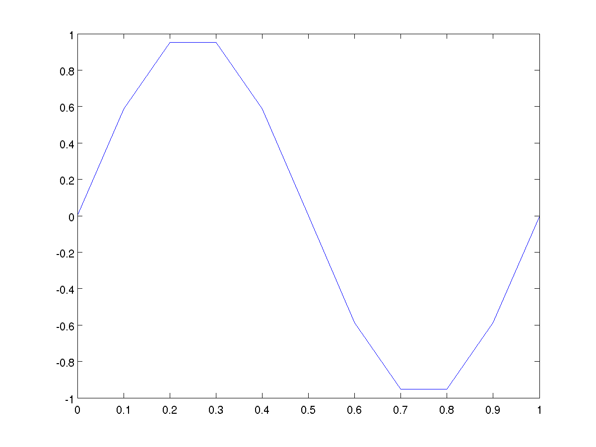
MATLAB actually plots the points (x(i), y(i)) joined by straight line segments. This becomes obvious if you do not use enough sample points when plotting a smooth function.
Create a vector x of 11 equally spaced points in [0, 1].
Create a vector y of function values.
Plot the points, producing the figure below.
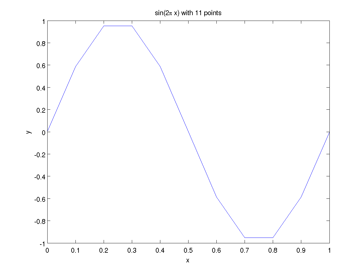
Title and labels
Every plot should have
- A title, which can be created with the title command;
- Axis labels, which can be created with the xlabel and ylabel commands;
Add a title. Note the use of \pi to get the mathematical symbol for pi in the title.
Add a label on the x-axis.
Add a label on the y-axis.
Line type and symbols
It is easy to change the line type by adding one of the following strings after the two vectors to be plotted: '-' (solid line), '--' (dashed line), ':' (dotted line), or '-.' (dash-dots).
It is also easy to plot a variety of symbols in a variety of colours at each of the data points. This will be very useful when plotting more than one set of data in the next module.
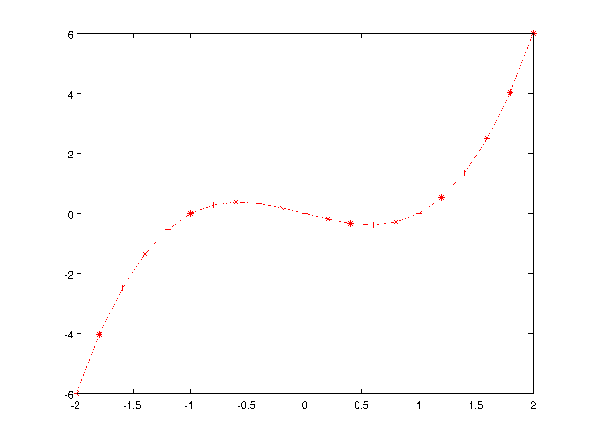
Create a vector of 21 points on [-2, 2].
Create a vector of polynomial values. Note use of .^ to get elementwise powers.
Plot with red stars joined by dashed lines, giving the figure below.
As always, more information can be obtained by typing
help plot
in the MATLAB command window, or using
doc plot
or the Help menu to open the MATLAB help browser.
Grids
Frequently it is useful to have a background grid, particularly when trying to read off values. This is achieved with the command
grid on
to turn the grid on, or
grid off
to turn the grid off.
Turn the grid on.

This plot should still have a title and axis labels added.
Warnings
- It is possible to customise almost any aspect of a plot using MATLAB's system of "handle graphics". However this can get quite complicated.
Self-test Exercise
Create a plot of the function f(x) = x e-x2 using 1001 equally spaced points on the interval [-5, 5]. Add a grid, title and axis labels.Answer:
x = linspace(-5, 5, 1001);
f = x .* exp(-x.^2);
plot(x, f)
grid on
xlabel('x')
ylabel('f')
title('f(x) = x exp(-x^2)')
Use the mouse to select the text between the word "Answer" and here to see the answer.
Summary
Two dimensional plots are created using the plot command.
Plots should always have a title (the title command), and axis labels (the xlabel and ylabel) and possibly a grid (use grid on)
A variety of line types, symbols and colours can be used -- see help plot.