


Multiple plots
The plot command can plot several sets of vectors.
Create a vector x of 401 equally spaced points on [0, 1].
Create a vector y1 of function values.
Create a vector y2 of function values.
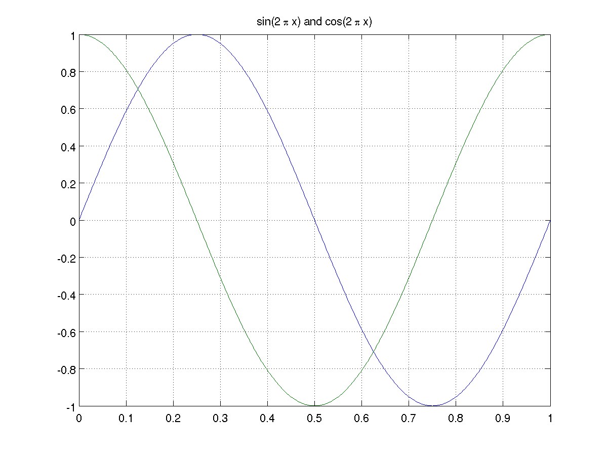
Plot both sets points in the same figure.
Add a grid.
Add a title. What is still missing?
In general you can use
plot(x1, y1, s1, x2, y2, s2, x3, y3, s3)
where x1 and y1 are vectors of the same length and s1 is an optional string.
Legends
When there are multiple plots in the same figure it is a good idea to add a legend, using, for example,
legend(string1, string2, string3)
Here string1 is a string describing the first set of values plotted, string2 is a string describing the second set of values plotted, and string3 is a string describing the third set of values plotted.
You can use the mouse to reposition the legend box within the plot, or you can specify the location of the legend box. See
help legendfor more information.

The hold command
If you have already created a plot and later wish to add another plot, then the hold command is useful.
Create the first plot assuming x, y1 and y2 are defined as above.
Turn the hold on.
Add the second plot.
Turn the hold off.
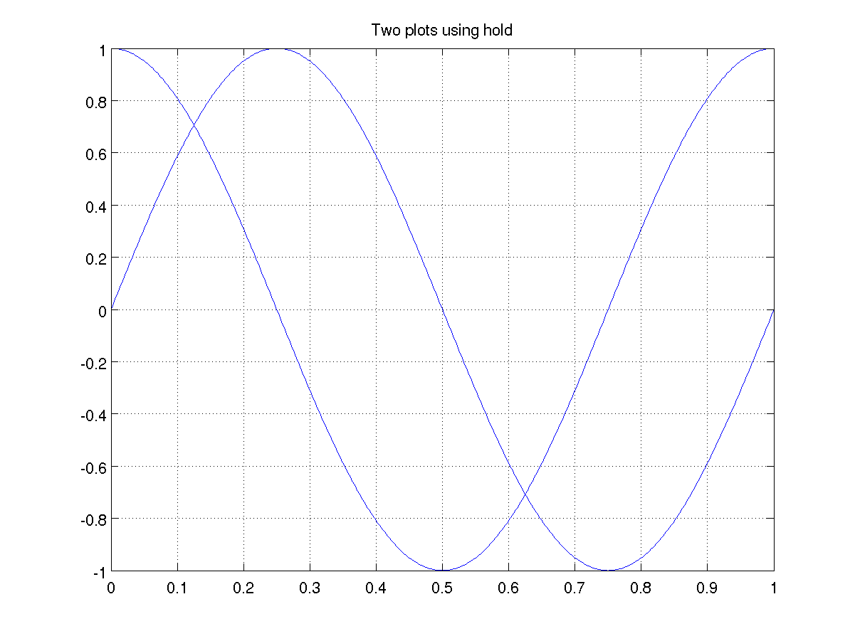
Note that when using a single plot command, MATLAB adjusts the colours for successive plots. When using the hold command you must explicitly set the colours, for example using plot(x, y2, 'g').
Subplots
Sometimes you want a single figure containing several individual subplots. The MATLAB command
subplot(m, n, k)
creates an m by n array of plots and positions you at plot number k, where the plots are numbered counting across rows.The most common examples are
- a 2 by 1 grid of subplots for two plots one on top of each other;
- a 1 by 2 grid for two plots side by side.
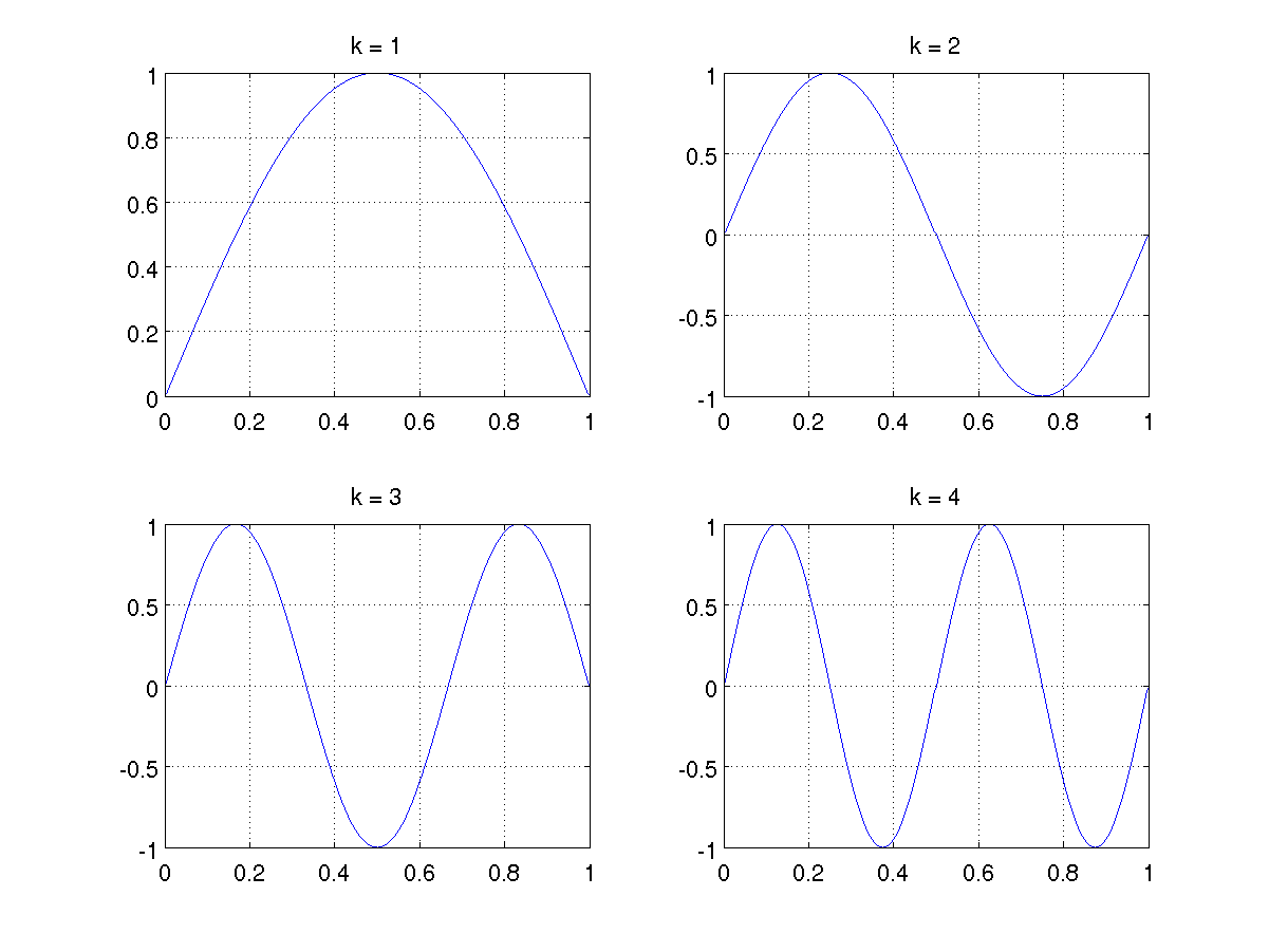
Here is a 2 by 2 grid of subplots to make it clear how the numbering of subplots works.
Create vector of plot points.
2 by 2 grid of subplots, at subplot 1.
Add plot on current subplot.
Add grid and title on current subplot.
2 by 2 grid of subplots, at subplot 2.
Add plot on current subplot.
Add grid and title on current subplot.
2 by 2 grid of subplots, at subplot 3.
Add plot on current subplot.
Add grid and title on current subplot.
2 by 2 grid of subplots, at subplot 4.
Add plot on current subplot.
Add grid and title on current subplot.
Axis limits
If you are really observant you will have noticed that the limits of the y-axis on the first subplot is from 0 to 1, while the other three plots all have y ranging from -1 to 1. MATLAB tries to choose good axis limits based on the data that is being plotted. However sometimes you want to change the axis limits.
The simplest way to do this is to use
xlim([xmin xmax])
to make the x-axis run from xmin to xmax. To adjust the limits of the y-axis use
ylim([ymin ymax])
to make the y-axis run from ymin to ymax. Note that the argument to xlim and ylim is a two element vector giving the lower and upper limits for the axis.
Another way to control the limits and scaling of the axes is to use the axis command, for example
axis([xmin xmax ymin ymax])
By default the x-scale is slightly larger than the y-scale, so you get a rectangular plot on the screen. To make the axis scaling equal use
axis equal
which is required to make a circle look like a circle!
As always, more information can be obtained by typing
help axis
in the MATLAB command window.
Create vector t of parameter values.
Store the values of cos(t) and sin(t).
Plot the two curves.
Make the axis scaling equal.
Adjust the axis limits.
Add a grid.

Figures
MATLAB draws a plot in the current figure window. Figure windows are labelled 1, 2, 3, ... The command
figure
creates a new figure window. Alternatively the commandfigure(k)
where k is a positive integer, opens figure window k if it already exists, or creates figure window k if it does not exist.
Self-test Exercise
Plot the functions sin(x), x, and 2x/pi over the interval [0, pi/2], including the title "Bounds on sin(x)", a grid, a legend and making sure the x-axis corresponds to the plot interval.Answer:
x = linspace(0, pi/2, 401);
plot(x, sin(x), x, x, x, 2*x/pi);
title('Bounds on sin(x)')
grid on
legend('sin(x)', 'x', '2x/pi')
xlim([0, pi/2])
Use the mouse to select the text between the word "Answer" and here to see the answer.
Summary
The plot command can plot several sets of data on the one set of axes. In this case a legend should be added.
Several different plots within the one figure can be created using the subplot command.
Axis limits and scaling can be modified with the xlim, ylim and axis commands.